Predicción 1 paso adelante usando 2 retardos

Vamos a importar la bases de datos y a convertirlas en objetos de series de Tiempo. \(\{X_t\}\)

Code

# get working directory
import os
os.getcwd()

'C:\\Users\\dofca\\Desktop\\series'

Code

# librerias
import pandas as pd
import numpy as np
import matplotlib.pylab as plt
import sklearn
import openpyxl
from skforecast.ForecasterAutoreg import ForecasterAutoreg
import warnings
print(f"Matplotlib Version: {plt.__version__}")
print(f"Pandas Version: {pd.__version__}")
print(f"Numpy Version: {np.__version__}")
print(f"Sklearn: {sklearn.__version__}")

Matplotlib Version: 1.25.2
Pandas Version: 2.0.3
Numpy Version: 1.25.2
Sklearn: 1.3.1

Code

# Lectura de la serie
data = pd.read_excel("datos/Exportaciones.xlsx",
                   header = 0, usecols = ['Mes','Total']).iloc[96:].reset_index(drop = True).round()
data['Total'] = data['Total'].astype(int) 
data

	Mes	Total
0	2000-01-01	1011676
1	2000-02-01	1054098
2	2000-03-01	1053546
3	2000-04-01	886359
4	2000-05-01	1146258
...	...	...
277	2023-02-01	4202234
278	2023-03-01	4431911
279	2023-04-01	3739214
280	2023-05-01	4497862
281	2023-06-01	3985981

282 rows × 2 columns

Code

# tipo de datos
print(data.info())

<class 'pandas.core.frame.DataFrame'>
RangeIndex: 282 entries, 0 to 281
Data columns (total 2 columns):
 #   Column  Non-Null Count  Dtype         
---  ------  --------------  -----         
 0   Mes     282 non-null    datetime64[ns]
 1   Total   282 non-null    int32         
dtypes: datetime64[ns](1), int32(1)
memory usage: 3.4 KB
None

Code

#mirando los datos
#objeto ts
exportaciones = data['Total']
print(type(exportaciones))
plt.plot(exportaciones)

<class 'pandas.core.series.Series'>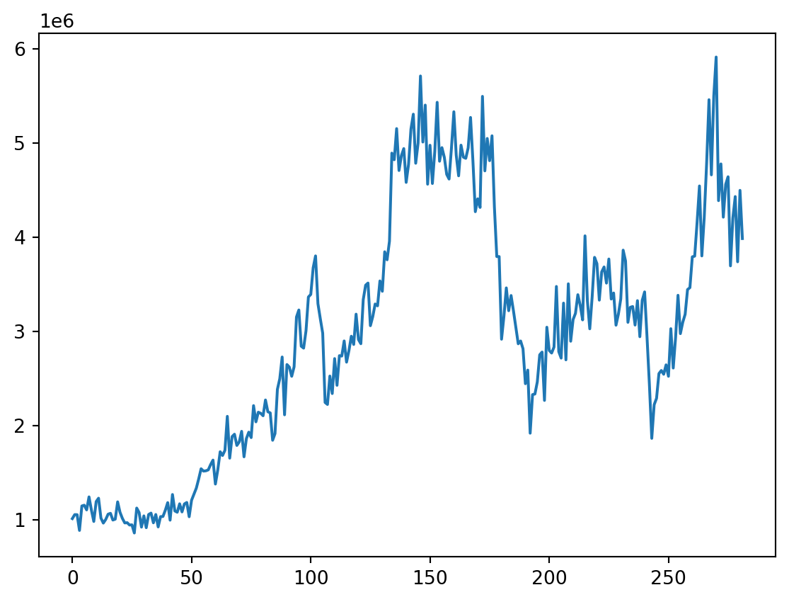

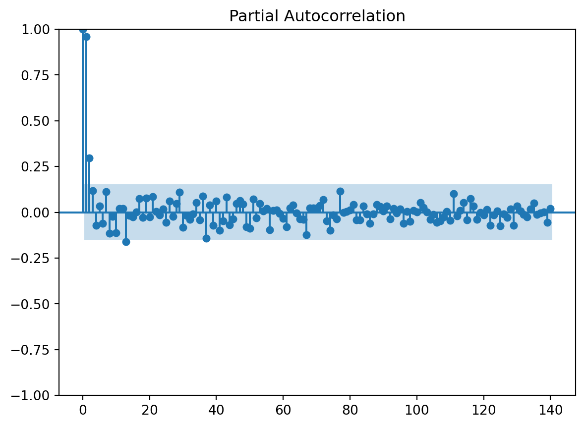
Code

print(f'Numero de filas con valores faltantes: {data.isnull().any(axis=1).mean()}')

Numero de filas con valores faltantes: 0.0

Code

data.shape

(282, 2)

0.1 PACF

usaremos la funcion de autocorrealcion parcial para darnos una idea de cuantos rezagos usaremos en el modelo

Code

from matplotlib import pyplot
from statsmodels.graphics.tsaplots import plot_pacf
plot_pacf(exportaciones,lags=140,method='ywm',alpha=0.01)
pyplot.show()

Code

import statsmodels.api as sm
pacf =  sm.tsa.stattools.pacf(exportaciones, nlags=140,method='ywm')
T = len(exportaciones)

sig_test = lambda tau_h: np.abs(tau_h) > 2.58/np.sqrt(T)

Code

pacf

array([ 1.00000000e+00,  9.59093603e-01,  2.97306056e-01,  1.17473996e-01,
       -7.03116609e-02,  3.26288216e-02, -6.03088214e-02,  1.13079878e-01,
       -1.13945940e-01, -2.33175139e-02, -1.11985646e-01,  2.02110227e-02,
        1.97278486e-02, -1.61423863e-01, -1.73791666e-02, -2.59991629e-02,
        2.41560086e-04,  7.51378723e-02, -2.72384453e-02,  7.60706013e-02,
       -2.47900629e-02,  8.49355502e-02,  3.74581253e-03, -1.43352938e-02,
        1.70410088e-02, -5.48238243e-02,  6.18273478e-02, -2.33524022e-02,
        4.74134619e-02,  1.08676085e-01, -8.12916663e-02, -1.67238998e-02,
       -3.96609731e-02, -1.05509554e-02,  5.15184774e-02, -4.09772449e-02,
        8.88414578e-02, -1.42772584e-01,  4.04045194e-02, -7.10728718e-02,
        6.10028381e-02, -9.75167769e-02, -4.70334839e-02,  8.36344066e-02,
       -6.77084813e-02, -3.56866811e-02,  4.65635129e-02,  6.27645281e-02,
        4.39629333e-02, -7.92100171e-02, -8.88109850e-02,  7.12681174e-02,
       -3.21905999e-02,  4.85459580e-02,  6.50733823e-03,  2.13679789e-02,
       -9.51162538e-02,  9.82890285e-03,  1.33457048e-02, -6.80490500e-03,
       -3.46524136e-02, -7.92901439e-02,  2.19653527e-02,  4.03653681e-02,
       -4.80582281e-03, -3.71454463e-02, -3.98280807e-02, -1.23770212e-01,
        2.30426145e-02,  2.40775563e-02,  2.36460653e-02,  3.65899044e-02,
        6.89818169e-02, -4.65605372e-02, -9.87423014e-02, -1.44166098e-02,
       -3.74822317e-02,  1.14862473e-01, -1.62496570e-03,  4.79499922e-03,
        1.21842509e-02,  4.07497124e-02, -4.06867111e-02, -4.16711832e-02,
        3.49704696e-02, -9.46634772e-03, -5.98154753e-02, -9.68932715e-03,
        4.16318031e-02,  3.05359681e-02,  5.76540164e-03,  3.41372435e-02,
       -3.61253646e-02,  2.07301731e-02, -4.34001846e-03,  1.87940224e-02,
       -5.97117781e-02,  3.06439973e-03, -4.93934874e-02,  1.06724162e-02,
        1.20967188e-03,  5.28574452e-02,  2.65553192e-02,  8.33244420e-04,
       -3.98366077e-02, -1.20608182e-02, -5.61664842e-02, -4.74597336e-02,
       -2.63848485e-02,  3.65173396e-03, -4.37024075e-02,  1.02159583e-01,
       -1.92846099e-02,  9.42032935e-03,  5.17064189e-02, -4.24857437e-02,
        7.57797502e-02,  3.32127608e-02, -3.92237359e-02, -1.64670791e-03,
       -1.41737394e-02,  1.55365471e-02, -7.03132739e-02, -1.44528291e-02,
        5.83931996e-03, -7.49281785e-02, -1.00802917e-02, -2.71361284e-02,
        1.70813154e-02, -7.28848521e-02,  3.34594698e-02,  5.60933395e-03,
       -1.26753457e-02, -2.48107506e-02,  1.84242234e-02,  4.94408804e-02,
       -1.08315454e-02, -4.22730382e-03,  1.63697862e-03, -5.47095096e-02,
        1.97184305e-02])

Code

for i in range(len(pacf)):
    if sig_test(pacf[i]) == False:
        n_steps = i - 1
        print('n_steps set to', n_steps)
        break

n_steps set to 2

Observamos que con el pacf se nos recomienda usar dos retardos, lo cuál nos recueda que cuando se quizo establecer una componente estacional se sugeria un periodo de 2.4, por lo tanto teniendo encuenta lo anterior usaremos 2 retrasos para la serie original

1 Árboles de decisión

1.0.1 Creación de los rezagos

Debido al análisis previo tomaremos los rezagos de 2 días atrás para poder predecir un paso adelante.

Code

from pandas import DataFrame
# reframe as supervised learning
# lag observation (t-1) is the input variable and t is the output variable.
df1 = DataFrame() # original
print(df1)
df2 = DataFrame() #diferenciada
print(df2)

Empty DataFrame
Columns: []
Index: []
Empty DataFrame
Columns: []
Index: []

Code

# arreglo de datos para el arreglo de rezagos Serie Original
indice = pd.date_range(start='1/1/2000', periods=282, freq='M')
print(indice)
originalDatadf = pd.DataFrame(data['Total'].values,index=indice)
print(originalDatadf)

DatetimeIndex(['2000-01-31', '2000-02-29', '2000-03-31', '2000-04-30',
               '2000-05-31', '2000-06-30', '2000-07-31', '2000-08-31',
               '2000-09-30', '2000-10-31',
               ...
               '2022-09-30', '2022-10-31', '2022-11-30', '2022-12-31',
               '2023-01-31', '2023-02-28', '2023-03-31', '2023-04-30',
               '2023-05-31', '2023-06-30'],
              dtype='datetime64[ns]', length=282, freq='M')
                  0
2000-01-31  1011676
2000-02-29  1054098
2000-03-31  1053546
2000-04-30   886359
2000-05-31  1146258
...             ...
2023-02-28  4202234
2023-03-31  4431911
2023-04-30  3739214
2023-05-31  4497862
2023-06-30  3985981

[282 rows x 1 columns]

Code

# Rezagos original
for i in range(2,0,-1):
    df1[['t-'+str(i)]] = originalDatadf.shift(i)
print(df1)

                  t-2        t-1
2000-01-31        NaN        NaN
2000-02-29        NaN  1011676.0
2000-03-31  1011676.0  1054098.0
2000-04-30  1054098.0  1053546.0
2000-05-31  1053546.0   886359.0
...               ...        ...
2023-02-28  4642084.0  3696188.0
2023-03-31  3696188.0  4202234.0
2023-04-30  4202234.0  4431911.0
2023-05-31  4431911.0  3739214.0
2023-06-30  3739214.0  4497862.0

[282 rows x 2 columns]

Code

# Create column t original
df1['t'] = originalDatadf.values
print(df1.head(14))

                  t-2        t-1        t
2000-01-31        NaN        NaN  1011676
2000-02-29        NaN  1011676.0  1054098
2000-03-31  1011676.0  1054098.0  1053546
2000-04-30  1054098.0  1053546.0   886359
2000-05-31  1053546.0   886359.0  1146258
2000-06-30   886359.0  1146258.0  1153956
2000-07-31  1146258.0  1153956.0  1104408
2000-08-31  1153956.0  1104408.0  1242391
2000-09-30  1104408.0  1242391.0  1102913
2000-10-31  1242391.0  1102913.0   981716
2000-11-30  1102913.0   981716.0  1192681
2000-12-31   981716.0  1192681.0  1228398
2001-01-31  1192681.0  1228398.0  1017195
2001-02-28  1228398.0  1017195.0   964437

Code

# Create a new subsetted dataframe, removing Nans from first 3 rows original
df1_Ori = df1[2:]
print(df1_Ori)
df1_Ori.size

                  t-2        t-1        t
2000-03-31  1011676.0  1054098.0  1053546
2000-04-30  1054098.0  1053546.0   886359
2000-05-31  1053546.0   886359.0  1146258
2000-06-30   886359.0  1146258.0  1153956
2000-07-31  1146258.0  1153956.0  1104408
...               ...        ...      ...
2023-02-28  4642084.0  3696188.0  4202234
2023-03-31  3696188.0  4202234.0  4431911
2023-04-30  4202234.0  4431911.0  3739214
2023-05-31  4431911.0  3739214.0  4497862
2023-06-30  3739214.0  4497862.0  3985981

[280 rows x 3 columns]

Code

# Split data Serie Original
Orig_Split = df1_Ori.values
# split into lagged variables and original time series
X1 = Orig_Split[:, 0:-1]  # slice all rows and start with column 0 and go up to but not including the last column
y1 = Orig_Split[:,-1]  # slice all rows and last column, essentially separating out 't' column
print(X1)
print('Respuestas \n',y1)

[[1011676. 1054098.]
 [1054098. 1053546.]
 [1053546.  886359.]
 [ 886359. 1146258.]
 [1146258. 1153956.]
 [1153956. 1104408.]
 [1104408. 1242391.]
 [1242391. 1102913.]
 [1102913.  981716.]
 [ 981716. 1192681.]
 [1192681. 1228398.]
 [1228398. 1017195.]
 [1017195.  964437.]
 [ 964437. 1002450.]
 [1002450. 1058457.]
 [1058457. 1068023.]
 [1068023.  996736.]
 [ 996736. 1005867.]
 [1005867. 1189605.]
 [1189605. 1078781.]
 [1078781. 1013772.]
 [1013772.  965973.]
 [ 965973.  968599.]
 [ 968599.  943702.]
 [ 943702.  945935.]
 [ 945935.  859303.]
 [ 859303. 1123902.]
 [1123902. 1076509.]
 [1076509.  921463.]
 [ 921463. 1040876.]
 [1040876.  915457.]
 [ 915457. 1055414.]
 [1055414. 1070342.]
 [1070342.  966897.]
 [ 966897. 1055590.]
 [1055590.  923427.]
 [ 923427. 1033043.]
 [1033043. 1034233.]
 [1034233. 1101056.]
 [1101056. 1181888.]
 [1181888.  995297.]
 [ 995297. 1267598.]
 [1267598. 1092850.]
 [1092850. 1079472.]
 [1079472. 1169195.]
 [1169195. 1082836.]
 [1082836. 1167628.]
 [1167628. 1183399.]
 [1183399. 1031826.]
 [1031826. 1206657.]
 [1206657. 1271618.]
 [1271618. 1335727.]
 [1335727. 1433647.]
 [1433647. 1541103.]
 [1541103. 1516523.]
 [1516523. 1519458.]
 [1519458. 1529291.]
 [1529291. 1585709.]
 [1585709. 1633370.]
 [1633370. 1378980.]
 [1378980. 1529265.]
 [1529265. 1722081.]
 [1722081. 1682450.]
 [1682450. 1737198.]
 [1737198. 2097853.]
 [2097853. 1653833.]
 [1653833. 1882740.]
 [1882740. 1908016.]
 [1908016. 1788905.]
 [1788905. 1826199.]
 [1826199. 1938567.]
 [1938567. 1668171.]
 [1668171. 1862024.]
 [1862024. 1929864.]
 [1929864. 1872161.]
 [1872161. 2211681.]
 [2211681. 2039364.]
 [2039364. 2141958.]
 [2141958. 2129881.]
 [2129881. 2104243.]
 [2104243. 2271572.]
 [2271572. 2146547.]
 [2146547. 2134504.]
 [2134504. 1843668.]
 [1843668. 1914770.]
 [1914770. 2384657.]
 [2384657. 2497750.]
 [2497750. 2727980.]
 [2727980. 2114259.]
 [2114259. 2648147.]
 [2648147. 2621002.]
 [2621002. 2523170.]
 [2523170. 2623649.]
 [2623649. 3152653.]
 [3152653. 3227536.]
 [3227536. 2842306.]
 [2842306. 2822470.]
 [2822470. 3007288.]
 [3007288. 3365420.]
 [3365420. 3392615.]
 [3392615. 3675654.]
 [3675654. 3801685.]
 [3801685. 3294187.]
 [3294187. 3133994.]
 [3133994. 2981105.]
 [2981105. 2245379.]
 [2245379. 2224271.]
 [2224271. 2525698.]
 [2525698. 2340118.]
 [2340118. 2711332.]
 [2711332. 2427571.]
 [2427571. 2742519.]
 [2742519. 2738083.]
 [2738083. 2898600.]
 [2898600. 2673470.]
 [2673470. 2795983.]
 [2795983. 2948687.]
 [2948687. 2861294.]
 [2861294. 3182972.]
 [3182972. 2913433.]
 [2913433. 2869156.]
 [2869156. 3337903.]
 [3337903. 3490978.]
 [3490978. 3513331.]
 [3513331. 3060628.]
 [3060628. 3157626.]
 [3157626. 3291236.]
 [3291236. 3271661.]
 [3271661. 3535759.]
 [3535759. 3426095.]
 [3426095. 3845531.]
 [3845531. 3760176.]
 [3760176. 3958572.]
 [3958572. 4893312.]
 [4893312. 4823094.]
 [4823094. 5153710.]
 [5153710. 4708737.]
 [4708737. 4866229.]
 [4866229. 4941645.]
 [4941645. 4582401.]
 [4582401. 4772996.]
 [4772996. 5147330.]
 [5147330. 5306738.]
 [5306738. 4785773.]
 [4785773. 4999318.]
 [4999318. 5712355.]
 [5712355. 5010929.]
 [5010929. 5403375.]
 [5403375. 4563431.]
 [4563431. 4976905.]
 [4976905. 4570780.]
 [4570780. 4910403.]
 [4910403. 5432930.]
 [5432930. 4807338.]
 [4807338. 4951628.]
 [4951628. 4849196.]
 [4849196. 4667767.]
 [4667767. 4617842.]
 [4617842. 4949487.]
 [4949487. 5332470.]
 [5332470. 4870839.]
 [4870839. 4652297.]
 [4652297. 4977706.]
 [4977706. 4849996.]
 [4849996. 4837983.]
 [4837983. 4948665.]
 [4948665. 5272122.]
 [5272122. 4808832.]
 [4808832. 4271442.]
 [4271442. 4408181.]
 [4408181. 4316676.]
 [4316676. 5495867.]
 [5495867. 4704814.]
 [4704814. 5048930.]
 [5048930. 4813091.]
 [4813091. 5077247.]
 [5077247. 4322278.]
 [4322278. 3794686.]
 [3794686. 3794711.]
 [3794711. 2916976.]
 [2916976. 3160957.]
 [3160957. 3461944.]
 [3461944. 3219706.]
 [3219706. 3381084.]
 [3381084. 3217408.]
 [3217408. 3043778.]
 [3043778. 2868451.]
 [2868451. 2898168.]
 [2898168. 2815522.]
 [2815522. 2444535.]
 [2444535. 2588994.]
 [2588994. 1919053.]
 [1919053. 2328723.]
 [2328723. 2334998.]
 [2334998. 2463793.]
 [2463793. 2751470.]
 [2751470. 2780512.]
 [2780512. 2266997.]
 [2266997. 3044377.]
 [3044377. 2797686.]
 [2797686. 2770014.]
 [2770014. 2833622.]
 [2833622. 3477094.]
 [3477094. 2785044.]
 [2785044. 2716024.]
 [2716024. 3300421.]
 [3300421. 2697992.]
 [2697992. 3505436.]
 [3505436. 2895612.]
 [2895612. 3125483.]
 [3125483. 3191598.]
 [3191598. 3389679.]
 [3389679. 3277516.]
 [3277516. 3122237.]
 [3122237. 4014818.]
 [4014818. 3324889.]
 [3324889. 3027603.]
 [3027603. 3365116.]
 [3365116. 3786537.]
 [3786537. 3719410.]
 [3719410. 3331933.]
 [3331933. 3632055.]
 [3632055. 3684399.]
 [3684399. 3512842.]
 [3512842. 3768666.]
 [3768666. 3343509.]
 [3343509. 3407819.]
 [3407819. 3066110.]
 [3066110. 3183071.]
 [3183071. 3344850.]
 [3344850. 3862819.]
 [3862819. 3748342.]
 [3748342. 3096363.]
 [3096363. 3255830.]
 [3255830. 3264261.]
 [3264261. 3067349.]
 [3067349. 3326497.]
 [3326497. 2943625.]
 [2943625. 3330051.]
 [3330051. 3419466.]
 [3419466. 2943626.]
 [2943626. 2439036.]
 [2439036. 1864239.]
 [1864239. 2221172.]
 [2221172. 2289482.]
 [2289482. 2551988.]
 [2551988. 2584767.]
 [2584767. 2544874.]
 [2544874. 2644954.]
 [2644954. 2523372.]
 [2523372. 3028837.]
 [3028837. 2610936.]
 [2610936. 2938994.]
 [2938994. 3383554.]
 [3383554. 2976372.]
 [2976372. 3096913.]
 [3096913. 3182216.]
 [3182216. 3444158.]
 [3444158. 3465143.]
 [3465143. 3792236.]
 [3792236. 3799111.]
 [3799111. 4155805.]
 [4155805. 4544551.]
 [4544551. 3801609.]
 [3801609. 4209198.]
 [4209198. 4780210.]
 [4780210. 5460531.]
 [5460531. 4662521.]
 [4662521. 5497617.]
 [5497617. 5913682.]
 [5913682. 4388737.]
 [4388737. 4778520.]
 [4778520. 4213182.]
 [4213182. 4562248.]
 [4562248. 4642084.]
 [4642084. 3696188.]
 [3696188. 4202234.]
 [4202234. 4431911.]
 [4431911. 3739214.]
 [3739214. 4497862.]]
Respuestas 
 [1053546.  886359. 1146258. 1153956. 1104408. 1242391. 1102913.  981716.
 1192681. 1228398. 1017195.  964437. 1002450. 1058457. 1068023.  996736.
 1005867. 1189605. 1078781. 1013772.  965973.  968599.  943702.  945935.
  859303. 1123902. 1076509.  921463. 1040876.  915457. 1055414. 1070342.
  966897. 1055590.  923427. 1033043. 1034233. 1101056. 1181888.  995297.
 1267598. 1092850. 1079472. 1169195. 1082836. 1167628. 1183399. 1031826.
 1206657. 1271618. 1335727. 1433647. 1541103. 1516523. 1519458. 1529291.
 1585709. 1633370. 1378980. 1529265. 1722081. 1682450. 1737198. 2097853.
 1653833. 1882740. 1908016. 1788905. 1826199. 1938567. 1668171. 1862024.
 1929864. 1872161. 2211681. 2039364. 2141958. 2129881. 2104243. 2271572.
 2146547. 2134504. 1843668. 1914770. 2384657. 2497750. 2727980. 2114259.
 2648147. 2621002. 2523170. 2623649. 3152653. 3227536. 2842306. 2822470.
 3007288. 3365420. 3392615. 3675654. 3801685. 3294187. 3133994. 2981105.
 2245379. 2224271. 2525698. 2340118. 2711332. 2427571. 2742519. 2738083.
 2898600. 2673470. 2795983. 2948687. 2861294. 3182972. 2913433. 2869156.
 3337903. 3490978. 3513331. 3060628. 3157626. 3291236. 3271661. 3535759.
 3426095. 3845531. 3760176. 3958572. 4893312. 4823094. 5153710. 4708737.
 4866229. 4941645. 4582401. 4772996. 5147330. 5306738. 4785773. 4999318.
 5712355. 5010929. 5403375. 4563431. 4976905. 4570780. 4910403. 5432930.
 4807338. 4951628. 4849196. 4667767. 4617842. 4949487. 5332470. 4870839.
 4652297. 4977706. 4849996. 4837983. 4948665. 5272122. 4808832. 4271442.
 4408181. 4316676. 5495867. 4704814. 5048930. 4813091. 5077247. 4322278.
 3794686. 3794711. 2916976. 3160957. 3461944. 3219706. 3381084. 3217408.
 3043778. 2868451. 2898168. 2815522. 2444535. 2588994. 1919053. 2328723.
 2334998. 2463793. 2751470. 2780512. 2266997. 3044377. 2797686. 2770014.
 2833622. 3477094. 2785044. 2716024. 3300421. 2697992. 3505436. 2895612.
 3125483. 3191598. 3389679. 3277516. 3122237. 4014818. 3324889. 3027603.
 3365116. 3786537. 3719410. 3331933. 3632055. 3684399. 3512842. 3768666.
 3343509. 3407819. 3066110. 3183071. 3344850. 3862819. 3748342. 3096363.
 3255830. 3264261. 3067349. 3326497. 2943625. 3330051. 3419466. 2943626.
 2439036. 1864239. 2221172. 2289482. 2551988. 2584767. 2544874. 2644954.
 2523372. 3028837. 2610936. 2938994. 3383554. 2976372. 3096913. 3182216.
 3444158. 3465143. 3792236. 3799111. 4155805. 4544551. 3801609. 4209198.
 4780210. 5460531. 4662521. 5497617. 5913682. 4388737. 4778520. 4213182.
 4562248. 4642084. 3696188. 4202234. 4431911. 3739214. 4497862. 3985981.]

2 Árbol para Serie Original

2.0.0.1 Entrenamiento, Validación y prueba

Code

Y1 = y1
print('Complete Observations for Target after Supervised configuration: %d' %len(Y1))
traintarget_size = int(len(Y1) * 0.70) 
valtarget_size = int(len(Y1) * 0.10)+1# Set split
testtarget_size = int(len(Y1) * 0.20)# Set split
print(traintarget_size,valtarget_size,testtarget_size)
print('Train + Validation + Test: %d' %(traintarget_size+valtarget_size+testtarget_size))

Complete Observations for Target after Supervised configuration: 280
196 29 56
Train + Validation + Test: 281

Code

# Target Train-Validation-Test split(70-10-20)
train_target, val_target,test_target = Y1[0:traintarget_size], Y1[(traintarget_size):(traintarget_size+valtarget_size)],Y1[(traintarget_size+valtarget_size):len(Y1)]

print('Observations for Target: %d' % (len(Y1)))
print('Training Observations for Target: %d' % (len(train_target)))
print('Validation Observations for Target: %d' % (len(val_target)))
print('Test Observations for Target: %d' % (len(test_target)))

Observations for Target: 280
Training Observations for Target: 196
Validation Observations for Target: 29
Test Observations for Target: 55

Code

# Features Train--Val-Test split

trainfeature_size = int(len(X1) * 0.70)
valfeature_size = int(len(X1) * 0.10)+1# Set split
testfeature_size = int(len(X1) * 0.20)# Set split
train_feature, val_feature,test_feature = X1[0:traintarget_size],X1[(traintarget_size):(traintarget_size+valtarget_size)] ,X1[(traintarget_size+valtarget_size):len(Y1)]

print('Observations for Feature: %d' % (len(X1)))
print('Training Observations for Feature: %d' % (len(train_feature)))
print('Validation Observations for Feature: %d' % (len(val_feature)))
print('Test Observations for Feature: %d' % (len(test_feature)))

Observations for Feature: 280
Training Observations for Feature: 196
Validation Observations for Feature: 29
Test Observations for Feature: 55

2.0.1 Árbol

Code

# Decision Tree Regresion Model
from sklearn.tree import DecisionTreeRegressor
# Create a decision tree regression model with default arguments
decision_tree_Orig = DecisionTreeRegressor()  # max-depth not set
# The maximum depth of the tree. If None, then nodes are expanded until all leaves are pure or until all leaves contain less than min_samples_split samples.
# Fit the model to the training features(covariables) and targets(respuestas)
decision_tree_Orig.fit(train_feature, train_target)
# Check the score on train and test
print("Coeficiente R2 sobre el conjunto de entrenamiento:",decision_tree_Orig.score(train_feature, train_target))
print("Coeficiente R2 sobre el conjunto de Validación:",decision_tree_Orig.score(val_feature,val_target))  # predictions are horrible if negative value, no relationship if 0
print("el RECM sobre validación es:",(((decision_tree_Orig.predict(val_feature)-val_target)**2).mean()) )

Coeficiente R2 sobre el conjunto de entrenamiento: 1.0
Coeficiente R2 sobre el conjunto de Validación: -0.9957468394345483
el RECM sobre validación es: 314021133770.5517

Vemos que el R2 para los datos de validación es bueno así sin ningún ajuste, Se relizara un ajuste de la profundidad como hiperparametro para ver si mejora dicho valor

Code

# Find the best Max Depth

# Loop through a few different max depths and check the performance
# Try different max depths. We want to optimize our ML models to make the best predictions possible.
# For regular decision trees, max_depth, which is a hyperparameter, limits the number of splits in a tree.
# You can find the best value of max_depth based on the R-squared score of the model on the test set.

for d in [2, 3, 4, 5,6,7,8,9,10,11,12,13,14,15]:
    # Create the tree and fit it
    decision_tree_Orig = DecisionTreeRegressor(max_depth=d)
    decision_tree_Orig.fit(train_feature, train_target)
    
    # Print out the scores on train and test
    print('max_depth=', str(d))
    print("Coeficiente R2 sobre el conjunto de entrenamiento:",decision_tree_Orig.score(train_feature, train_target))
    print("Coeficiente R2 sobre el conjunto de validación:",decision_tree_Orig.score(val_feature, val_target), '\n')  # You want the test score to be positive and high
    print("el RECM sobre el conjunto de validación es:",sklearn.metrics.mean_squared_error(decision_tree_Orig.predict(val_feature),val_target, squared=False))

max_depth= 2
Coeficiente R2 sobre el conjunto de entrenamiento: 0.9448886702102718
Coeficiente R2 sobre el conjunto de validación: -1.088017789994565 

el RECM sobre el conjunto de validación es: 573183.6726079404
max_depth= 3
Coeficiente R2 sobre el conjunto de entrenamiento: 0.9692432238418371
Coeficiente R2 sobre el conjunto de validación: -0.8422460453834877 

el RECM sobre el conjunto de validación es: 538394.3950459106
max_depth= 4
Coeficiente R2 sobre el conjunto de entrenamiento: 0.9783266474186452
Coeficiente R2 sobre el conjunto de validación: -0.5669014414580396 

el RECM sobre el conjunto de validación es: 496532.35543516674
max_depth= 5
Coeficiente R2 sobre el conjunto de entrenamiento: 0.9842654186860248
Coeficiente R2 sobre el conjunto de validación: -0.8380486254917823 

el RECM sobre el conjunto de validación es: 537780.6995918642
max_depth= 6
Coeficiente R2 sobre el conjunto de entrenamiento: 0.9897832765928137
Coeficiente R2 sobre el conjunto de validación: -0.9542318718699783 

el RECM sobre el conjunto de validación es: 554516.8653650281
max_depth= 7
Coeficiente R2 sobre el conjunto de entrenamiento: 0.9937044281888229
Coeficiente R2 sobre el conjunto de validación: -0.8843688632366069 

el RECM sobre el conjunto de validación es: 544514.7809955052
max_depth= 8
Coeficiente R2 sobre el conjunto de entrenamiento: 0.9965163518047335
Coeficiente R2 sobre el conjunto de validación: -1.0173859465570052 

el RECM sobre el conjunto de validación es: 563405.6645496098
max_depth= 9
Coeficiente R2 sobre el conjunto de entrenamiento: 0.997736780045468
Coeficiente R2 sobre el conjunto de validación: -0.958310123886982 

el RECM sobre el conjunto de validación es: 555095.1695408727
max_depth= 10
Coeficiente R2 sobre el conjunto de entrenamiento: 0.9991593867209211
Coeficiente R2 sobre el conjunto de validación: -1.1076259140640996 

el RECM sobre el conjunto de validación es: 575868.7057293948
max_depth= 11
Coeficiente R2 sobre el conjunto de entrenamiento: 0.9997209884655672
Coeficiente R2 sobre el conjunto de validación: -0.9499196090238338 

el RECM sobre el conjunto de validación es: 553904.721252913
max_depth= 12
Coeficiente R2 sobre el conjunto de entrenamiento: 0.9998998175749997
Coeficiente R2 sobre el conjunto de validación: -1.0445150478674257 

el RECM sobre el conjunto de validación es: 567181.2549913402
max_depth= 13
Coeficiente R2 sobre el conjunto de entrenamiento: 0.9999707138251954
Coeficiente R2 sobre el conjunto de validación: -0.9704446621528584 

el RECM sobre el conjunto de validación es: 556812.3187240271
max_depth= 14
Coeficiente R2 sobre el conjunto de entrenamiento: 0.9999969265889176
Coeficiente R2 sobre el conjunto de validación: -0.9506669786796578 

el RECM sobre el conjunto de validación es: 554010.8620188123
max_depth= 15
Coeficiente R2 sobre el conjunto de entrenamiento: 1.0
Coeficiente R2 sobre el conjunto de validación: -0.9300433322924266 

el RECM sobre el conjunto de validación es: 551074.4087733494

Note que los scores para el conjunto de validación son negativos para todas las profundidades evaluadas. Ahora uniremos validacion y entrenamiento para re para reestimar los parametros

Code

print(type(train_feature))
print(type(val_feature))
#######
print(type(train_target))
print(type(val_target))
####
print(train_feature.shape)
print(val_feature.shape)
#####
####
print(train_target.shape)
print(val_target.shape)
###Concatenate Validation and test
train_val_feature=np.concatenate((train_feature,val_feature),axis=0)
train_val_target=np.concatenate((train_target,val_target),axis=0)
print(train_val_feature.shape)
print(train_val_target.shape)

<class 'numpy.ndarray'>
<class 'numpy.ndarray'>
<class 'numpy.ndarray'>
<class 'numpy.ndarray'>
(196, 2)
(29, 2)
(196,)
(29,)
(225, 2)
(225,)

Code

# Use the best max_depth 
decision_tree_Orig = DecisionTreeRegressor(max_depth=4)  # fill in best max depth here
decision_tree_Orig.fit(train_val_feature, train_val_target)

# Predict values for train and test
train_val_prediction = decision_tree_Orig.predict(train_val_feature)
test_prediction = decision_tree_Orig.predict(test_feature)

# Scatter the predictions vs actual values
plt.scatter(train_val_prediction, train_val_target, label='train')  # blue
plt.scatter(test_prediction, test_target, label='test')  # orange
# Agrega títulos a los ejes
plt.xlabel('Valores Predichos')  # Título para el eje x
plt.ylabel('Valores Objetivo')  # Título para el eje y
# Muestra una leyenda
plt.legend()
plt.show()
print("Raíz de la Pérdida cuadrática Entrenamiento:",sklearn.metrics.mean_squared_error( train_val_prediction, train_val_target,squared=False))

print("Raíz de la Pérdida cuadrática Prueba:",sklearn.metrics.mean_squared_error(test_prediction, test_target,squared=False))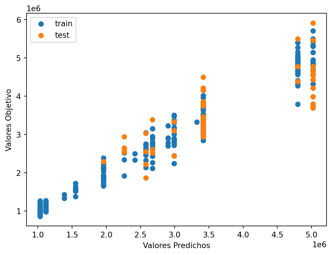

Raíz de la Pérdida cuadrática Entrenamiento: 249566.97518562482
Raíz de la Pérdida cuadrática Prueba: 552220.6310930281

Code

from sklearn import tree

listacaract=list(df1_Ori.columns.values)
respuesta=listacaract.pop()
text_representation = tree.export_text(decision_tree_Orig)
print(text_representation)

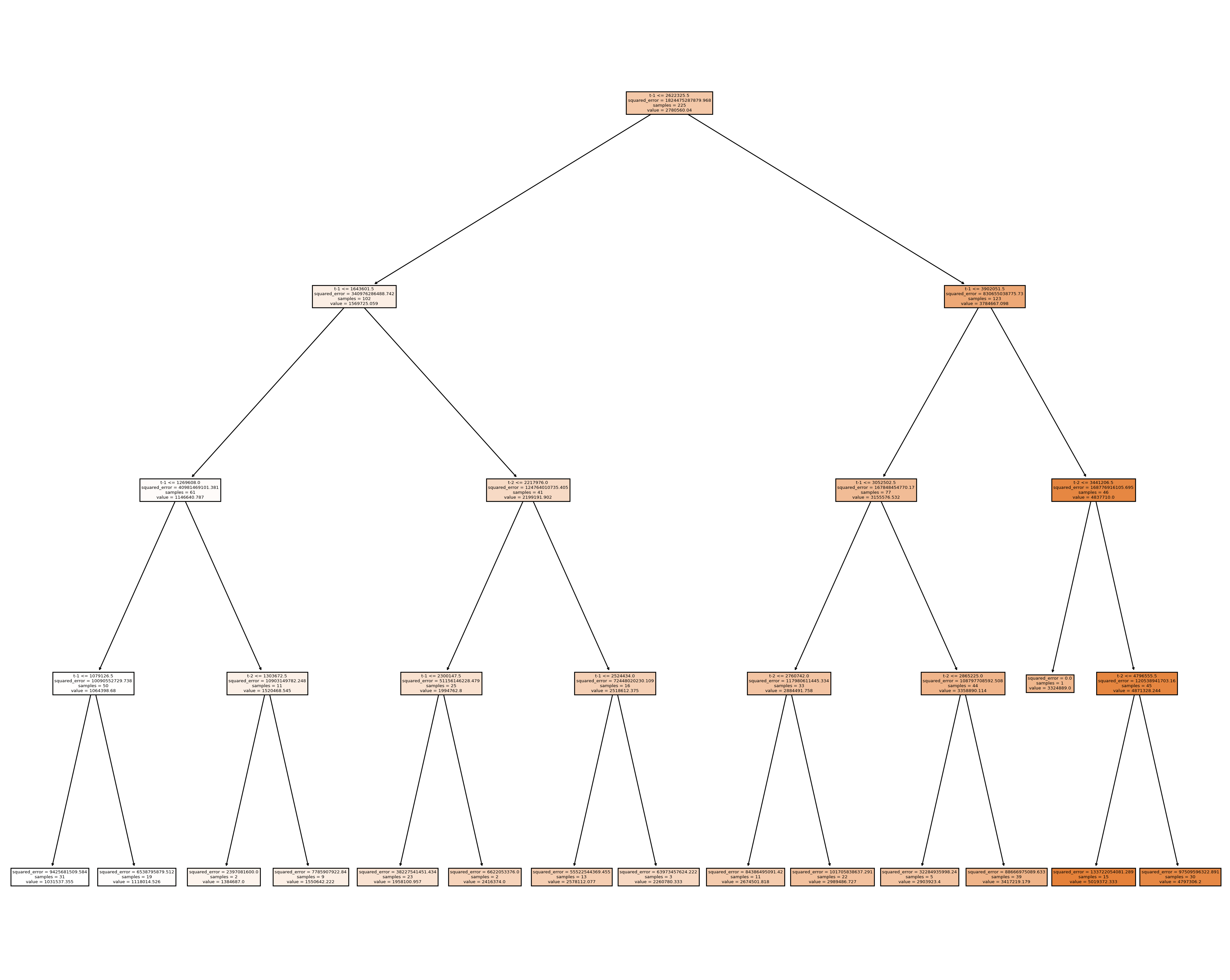
|--- feature_1 <= 2622325.50
|   |--- feature_1 <= 1643601.50
|   |   |--- feature_1 <= 1269608.00
|   |   |   |--- feature_1 <= 1079126.50
|   |   |   |   |--- value: [1031537.35]
|   |   |   |--- feature_1 >  1079126.50
|   |   |   |   |--- value: [1118014.53]
|   |   |--- feature_1 >  1269608.00
|   |   |   |--- feature_0 <= 1303672.50
|   |   |   |   |--- value: [1384687.00]
|   |   |   |--- feature_0 >  1303672.50
|   |   |   |   |--- value: [1550642.22]
|   |--- feature_1 >  1643601.50
|   |   |--- feature_0 <= 2217976.00
|   |   |   |--- feature_1 <= 2300147.50
|   |   |   |   |--- value: [1958100.96]
|   |   |   |--- feature_1 >  2300147.50
|   |   |   |   |--- value: [2416374.00]
|   |   |--- feature_0 >  2217976.00
|   |   |   |--- feature_1 <= 2524434.00
|   |   |   |   |--- value: [2578112.08]
|   |   |   |--- feature_1 >  2524434.00
|   |   |   |   |--- value: [2260780.33]
|--- feature_1 >  2622325.50
|   |--- feature_1 <= 3902051.50
|   |   |--- feature_1 <= 3052502.50
|   |   |   |--- feature_0 <= 2760742.00
|   |   |   |   |--- value: [2674501.82]
|   |   |   |--- feature_0 >  2760742.00
|   |   |   |   |--- value: [2989486.73]
|   |   |--- feature_1 >  3052502.50
|   |   |   |--- feature_0 <= 2865225.00
|   |   |   |   |--- value: [2903923.40]
|   |   |   |--- feature_0 >  2865225.00
|   |   |   |   |--- value: [3417219.18]
|   |--- feature_1 >  3902051.50
|   |   |--- feature_0 <= 3441206.50
|   |   |   |--- value: [3324889.00]
|   |   |--- feature_0 >  3441206.50
|   |   |   |--- feature_0 <= 4796555.50
|   |   |   |   |--- value: [5019372.33]
|   |   |   |--- feature_0 >  4796555.50
|   |   |   |   |--- value: [4797306.20]

Code

fig = plt.figure(figsize=(25,20))
_ = tree.plot_tree(decision_tree_Orig, 
                   feature_names=listacaract,  
                   class_names=[respuesta],
                   filled=True)

Ahora miraremos las predicciones comparadas con los valores verdaderos, para ver más claro lo anterior.

Code

print(train_val_prediction.size)
print(train_val_target.size)

print(test_prediction.size)
print(test_target.size)

Code

indicetrian_val_test=df1_Ori.index
print(indicetrian_val_test.size)  ###Tamaño del índice
indicetrain_val=indicetrian_val_test[0:225]
indicetest=indicetrian_val_test[225:280]

Code

print(indicetrain_val.size)
print(indicetest.size)

225
55

Code

targetjoint=np.concatenate((train_val_target,test_target))
predictionjoint=np.concatenate((train_val_prediction,test_prediction))
print(targetjoint.size)
print(predictionjoint.size)

280
280

Code

d = {'observado': targetjoint, 'Predicción': predictionjoint}
ObsvsPred1=pd.DataFrame(data=d,index=indicetrian_val_test)
ObsvsPred1.head(10)

	observado	Predicción
2000-03-31	1053546.0	1.031537e+06
2000-04-30	886359.0	1.031537e+06
2000-05-31	1146258.0	1.031537e+06
2000-06-30	1153956.0	1.118015e+06
2000-07-31	1104408.0	1.118015e+06
2000-08-31	1242391.0	1.118015e+06
2000-09-30	1102913.0	1.118015e+06
2000-10-31	981716.0	1.118015e+06
2000-11-30	1192681.0	1.031537e+06
2000-12-31	1228398.0	1.118015e+06

Code

#gráfico
ax = ObsvsPred1['observado'].plot(marker="o", figsize=(10, 6), linewidth=1, markersize=4)  # Ajusta el grosor de las líneas y puntos
ObsvsPred1['Predicción'].plot(marker="o", linewidth=1, markersize=2, ax=ax)  # Ajusta el grosor de las líneas y puntos
# Agrega una línea vertical roja
ax.axvline(x=indicetrian_val_test[223].date(), color='red', linewidth=0.5)  # Ajusta el grosor de la línea vertical
# Muestra una leyenda
plt.legend()
plt.show()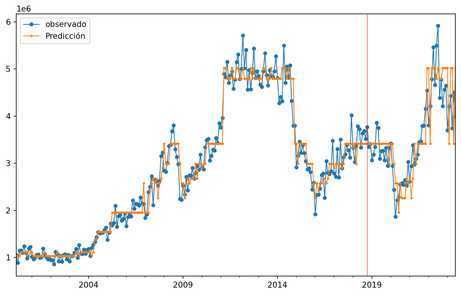

3 Serie de Exportaciones sin Tendencia

Implementaremos ahora el modelo de árboles sobre la serie sin tendencia, eliminada usando la estimación dada por medio del filtro de promedios móviles. Vamos a importar la bases de datos y a convertirlas en objetos de series de Tiempo. \(\{X_t\}\)

Code

# Lectura de la serie
data2 = pd.read_excel("ExportacionesSinTendencia.xlsx",
                   header = 0, usecols = ['Fecha','ExportacionesSinTend']).reset_index(drop = True).round()
data2['ExportacionesSinTend'] = data2['ExportacionesSinTend'].astype(int) 
data2

	Fecha	ExportacionesSinTend
0	2000-07-01	5
1	2000-08-01	70
2	2000-09-01	9
3	2000-10-01	-53
4	2000-11-01	46
...	...	...
265	2022-08-01	-71
266	2022-09-01	17
267	2022-10-01	-88
268	2022-11-01	7
269	2022-12-01	39

270 rows × 2 columns

Code

# tipo de datos
print(data2.info())

<class 'pandas.core.frame.DataFrame'>
RangeIndex: 270 entries, 0 to 269
Data columns (total 2 columns):
 #   Column                Non-Null Count  Dtype         
---  ------                --------------  -----         
 0   Fecha                 270 non-null    datetime64[ns]
 1   ExportacionesSinTend  270 non-null    int32         
dtypes: datetime64[ns](1), int32(1)
memory usage: 3.3 KB
None

Code

#mirando los datos
#objeto ts
exportaciones = data2['ExportacionesSinTend']
print(type(exportaciones))
plt.plot(exportaciones)

<class 'pandas.core.series.Series'>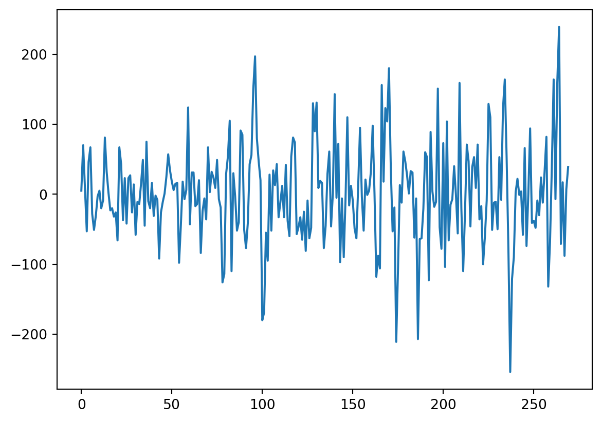

Code

print(f'Numero de filas con valores faltantes: {data2.isnull().any(axis=1).mean()}')

Numero de filas con valores faltantes: 0.0

Code

data2.shape

(270, 2)

3.1 PACF

usaremos la funcion de autocorrealcion parcial para darnos una idea de cuantos rezagos usaremos en el modelo

Code

from matplotlib import pyplot
from statsmodels.graphics.tsaplots import plot_pacf
plot_pacf(exportaciones,lags=134,method='ywm',alpha=0.01)
pyplot.show()

Code

import statsmodels.api as sm
pacf =  sm.tsa.stattools.pacf(exportaciones, nlags=134,method='ywm')
T = len(exportaciones)

sig_test = lambda tau_h: np.abs(tau_h) > 2.58/np.sqrt(T)

Code

pacf

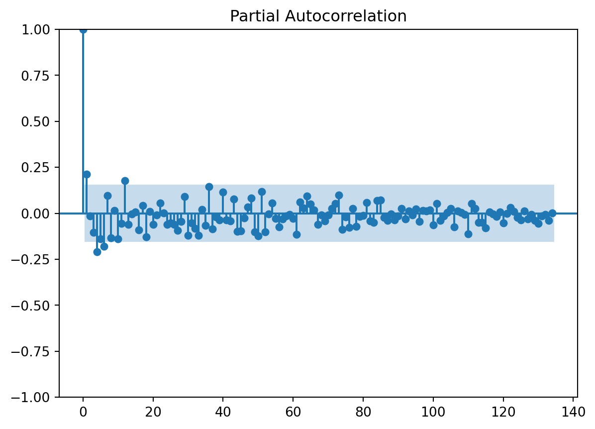
array([ 1.        ,  0.21355648, -0.01410819, -0.10451617, -0.2093758 ,
       -0.14017377, -0.17906702,  0.09686678, -0.13392601,  0.01595307,
       -0.13946366, -0.0563855 ,  0.17741868, -0.0609385 , -0.00478777,
        0.00611697, -0.09012201,  0.04079611, -0.1288755 ,  0.01040772,
       -0.06054336, -0.00809331,  0.05521414,  0.00145114, -0.06018931,
       -0.05344687, -0.06106559, -0.09355214, -0.04415682,  0.08980262,
       -0.12158518, -0.05246829, -0.08134046, -0.11923296,  0.01961602,
       -0.06611188,  0.14387345, -0.08387056, -0.02154623, -0.03719252,
        0.11636824, -0.03659881, -0.04184158,  0.0773012 , -0.09796869,
       -0.09592436, -0.02679615,  0.03304619,  0.08238835, -0.10051005,
       -0.1233177 ,  0.11816191, -0.10239664, -0.00298642,  0.05553658,
       -0.02902818, -0.07533038, -0.030158  , -0.01596098, -0.0076432 ,
       -0.02810041, -0.11429884,  0.06089394,  0.02933573,  0.09430358,
        0.04947294,  0.0168977 , -0.05976736, -0.00941411, -0.04209226,
       -0.00997868,  0.02671226,  0.05214744,  0.10015063, -0.08725013,
       -0.02096121, -0.07610181,  0.02608155, -0.07163182, -0.01742543,
       -0.01110346,  0.05773641, -0.0426505 , -0.04985717,  0.07024918,
        0.0724035 , -0.02324498, -0.03840519, -0.00384265, -0.03725229,
       -0.01497874,  0.02560091, -0.02994393,  0.01198395, -0.00979288,
        0.0224643 , -0.04398166,  0.01457101,  0.01353388,  0.01837122,
       -0.06478182,  0.05269882, -0.03988886, -0.01561551,  0.00534409,
        0.02551739, -0.07313363,  0.01118899,  0.0051652 , -0.00649134,
       -0.11102337,  0.05241729,  0.02498581, -0.05071817, -0.05116662,
       -0.07926453,  0.00801331, -0.00355665, -0.0184545 ,  0.00602772,
       -0.05354637, -0.00260395,  0.03088632,  0.00947186, -0.02269647,
       -0.03670284,  0.01269883, -0.02970479, -0.00677465, -0.03938635,
       -0.05408061, -0.01603313, -0.00598982, -0.03914117,  0.00226407])

Code

for i in range(len(pacf)):
    if sig_test(pacf[i]) == False:
        n_steps = i - 1
        print('n_steps set to', n_steps)
        break

n_steps set to 1

Observamos que con el pacf se nos recomienda usar un solo retardo, usaremos 1 retraso para la serie sin Tendencia

4 Árboles de decisión

4.0.1 Creación de los rezagos

Debido al análisis previo tomaremos los rezagos de 1 días atrás para poder predecir un paso adelante.

Code

from pandas import DataFrame
# reframe as supervised learning
# lag observation (t-1) is the input variable and t is the output variable.
df1 = DataFrame() # original
print(df1)
df2 = DataFrame() #diferenciada
print(df2)

Empty DataFrame
Columns: []
Index: []
Empty DataFrame
Columns: []
Index: []

Code

# arreglo de datos para el arreglo de rezagos Serie Original
indice = pd.date_range(start='1/7/2000', periods=270, freq='M')
print(indice)
originalDatadf = pd.DataFrame(data2['ExportacionesSinTend'].values,index=indice)
print(originalDatadf)

DatetimeIndex(['2000-01-31', '2000-02-29', '2000-03-31', '2000-04-30',
               '2000-05-31', '2000-06-30', '2000-07-31', '2000-08-31',
               '2000-09-30', '2000-10-31',
               ...
               '2021-09-30', '2021-10-31', '2021-11-30', '2021-12-31',
               '2022-01-31', '2022-02-28', '2022-03-31', '2022-04-30',
               '2022-05-31', '2022-06-30'],
              dtype='datetime64[ns]', length=270, freq='M')
             0
2000-01-31   5
2000-02-29  70
2000-03-31   9
2000-04-30 -53
2000-05-31  46
...         ..
2022-02-28 -71
2022-03-31  17
2022-04-30 -88
2022-05-31   7
2022-06-30  39

[270 rows x 1 columns]

Code

# Rezagos original
for i in range(1,0,-1):
    df1[['t-'+str(i)]] = originalDatadf.shift(i)
print(df1)

              t-1
2000-01-31    NaN
2000-02-29    5.0
2000-03-31   70.0
2000-04-30    9.0
2000-05-31  -53.0
...           ...
2022-02-28  239.0
2022-03-31  -71.0
2022-04-30   17.0
2022-05-31  -88.0
2022-06-30    7.0

[270 rows x 1 columns]

Code

# Create column t original
df1['t'] = originalDatadf.values
print(df1.head(14))

             t-1   t
2000-01-31   NaN   5
2000-02-29   5.0  70
2000-03-31  70.0   9
2000-04-30   9.0 -53
2000-05-31 -53.0  46
2000-06-30  46.0  67
2000-07-31  67.0 -28
2000-08-31 -28.0 -51
2000-09-30 -51.0 -31
2000-10-31 -31.0  -3
2000-11-30  -3.0   5
2000-12-31   5.0 -20
2001-01-31 -20.0  -9
2001-02-28  -9.0  81

Code

# Create a new subsetted dataframe, removing Nans from first 3 rows original
df1_Ori = df1[1:]
print(df1_Ori)
df1_Ori.size

              t-1   t
2000-02-29    5.0  70
2000-03-31   70.0   9
2000-04-30    9.0 -53
2000-05-31  -53.0  46
2000-06-30   46.0  67
...           ...  ..
2022-02-28  239.0 -71
2022-03-31  -71.0  17
2022-04-30   17.0 -88
2022-05-31  -88.0   7
2022-06-30    7.0  39

[269 rows x 2 columns]

Code

# Split data Serie Original
Orig_Split = df1_Ori.values
# split into lagged variables and original time series
X1 = Orig_Split[:, 0:-1]  # slice all rows and start with column 0 and go up to but not including the last column
y1 = Orig_Split[:,-1]  # slice all rows and last column, essentially separating out 't' column
print(X1)
print('Respuestas \n',y1)

[[   5.]
 [  70.]
 [   9.]
 [ -53.]
 [  46.]
 [  67.]
 [ -28.]
 [ -51.]
 [ -31.]
 [  -3.]
 [   5.]
 [ -20.]
 [  -9.]
 [  81.]
 [  32.]
 [   2.]
 [ -23.]
 [ -20.]
 [ -32.]
 [ -26.]
 [ -66.]
 [  67.]
 [  43.]
 [ -37.]
 [  23.]
 [ -42.]
 [  23.]
 [  27.]
 [ -26.]
 [  14.]
 [ -58.]
 [ -11.]
 [ -14.]
 [  15.]
 [  49.]
 [ -45.]
 [  75.]
 [ -10.]
 [ -20.]
 [  16.]
 [ -31.]
 [  -2.]
 [  -8.]
 [ -92.]
 [ -26.]
 [ -11.]
 [   1.]
 [  25.]
 [  57.]
 [  34.]
 [  18.]
 [   6.]
 [  15.]
 [  16.]
 [ -98.]
 [ -44.]
 [  18.]
 [  -7.]
 [   6.]
 [ 124.]
 [ -43.]
 [  31.]
 [  31.]
 [ -17.]
 [ -14.]
 [  20.]
 [ -84.]
 [ -24.]
 [  -6.]
 [ -36.]
 [  67.]
 [   3.]
 [  32.]
 [  24.]
 [   9.]
 [  49.]
 [  -7.]
 [ -19.]
 [-126.]
 [-114.]
 [  29.]
 [  54.]
 [ 105.]
 [-110.]
 [  30.]
 [  -3.]
 [ -52.]
 [ -40.]
 [  91.]
 [  85.]
 [ -51.]
 [ -77.]
 [ -41.]
 [  43.]
 [  56.]
 [ 150.]
 [ 197.]
 [  80.]
 [  47.]
 [  20.]
 [-180.]
 [-169.]
 [ -55.]
 [ -95.]
 [  28.]
 [ -52.]
 [  34.]
 [  13.]
 [  43.]
 [ -33.]
 [ -11.]
 [  12.]
 [ -33.]
 [  42.]
 [ -38.]
 [ -60.]
 [  54.]
 [  81.]
 [  74.]
 [ -57.]
 [ -47.]
 [ -33.]
 [ -65.]
 [ -25.]
 [ -81.]
 [  -9.]
 [ -63.]
 [ -48.]
 [ 130.]
 [  90.]
 [ 131.]
 [   9.]
 [  19.]
 [  16.]
 [ -77.]
 [ -45.]
 [  29.]
 [  61.]
 [ -46.]
 [   1.]
 [ 143.]
 [  -5.]
 [  72.]
 [ -97.]
 [  -6.]
 [ -90.]
 [  -6.]
 [ 110.]
 [ -16.]
 [  12.]
 [  -9.]
 [ -49.]
 [ -63.]
 [  13.]
 [  95.]
 [  -3.]
 [ -52.]
 [  21.]
 [  -1.]
 [   5.]
 [  32.]
 [  98.]
 [   1.]
 [-118.]
 [ -88.]
 [-106.]
 [ 156.]
 [  18.]
 [ 123.]
 [ 104.]
 [ 180.]
 [  38.]
 [ -53.]
 [ -19.]
 [-211.]
 [-106.]
 [  13.]
 [ -12.]
 [  61.]
 [  47.]
 [  27.]
 [   1.]
 [  33.]
 [  31.]
 [ -62.]
 [  -6.]
 [-207.]
 [ -64.]
 [ -63.]
 [ -21.]
 [  60.]
 [  53.]
 [-123.]
 [  89.]
 [   4.]
 [ -18.]
 [ -11.]
 [ 151.]
 [ -47.]
 [ -78.]
 [  73.]
 [-104.]
 [ 104.]
 [ -66.]
 [ -15.]
 [  -7.]
 [  40.]
 [  -1.]
 [ -56.]
 [ 159.]
 [ -20.]
 [-110.]
 [ -27.]
 [  71.]
 [  47.]
 [ -46.]
 [  39.]
 [  53.]
 [   9.]
 [  71.]
 [ -36.]
 [ -17.]
 [-100.]
 [ -61.]
 [  -9.]
 [ 129.]
 [ 110.]
 [ -51.]
 [ -12.]
 [ -11.]
 [ -50.]
 [  53.]
 [  -8.]
 [ 123.]
 [ 164.]
 [  54.]
 [ -79.]
 [-254.]
 [-121.]
 [ -90.]
 [   3.]
 [  22.]
 [  -1.]
 [   4.]
 [ -58.]
 [  66.]
 [ -74.]
 [   0.]
 [  94.]
 [ -41.]
 [ -38.]
 [ -48.]
 [  -9.]
 [ -30.]
 [  24.]
 [ -12.]
 [  33.]
 [  82.]
 [-132.]
 [ -68.]
 [  39.]
 [ 164.]
 [  -7.]
 [ 159.]
 [ 239.]
 [ -71.]
 [  17.]
 [ -88.]
 [   7.]]
Respuestas 
 [  70.    9.  -53.   46.   67.  -28.  -51.  -31.   -3.    5.  -20.   -9.
   81.   32.    2.  -23.  -20.  -32.  -26.  -66.   67.   43.  -37.   23.
  -42.   23.   27.  -26.   14.  -58.  -11.  -14.   15.   49.  -45.   75.
  -10.  -20.   16.  -31.   -2.   -8.  -92.  -26.  -11.    1.   25.   57.
   34.   18.    6.   15.   16.  -98.  -44.   18.   -7.    6.  124.  -43.
   31.   31.  -17.  -14.   20.  -84.  -24.   -6.  -36.   67.    3.   32.
   24.    9.   49.   -7.  -19. -126. -114.   29.   54.  105. -110.   30.
   -3.  -52.  -40.   91.   85.  -51.  -77.  -41.   43.   56.  150.  197.
   80.   47.   20. -180. -169.  -55.  -95.   28.  -52.   34.   13.   43.
  -33.  -11.   12.  -33.   42.  -38.  -60.   54.   81.   74.  -57.  -47.
  -33.  -65.  -25.  -81.   -9.  -63.  -48.  130.   90.  131.    9.   19.
   16.  -77.  -45.   29.   61.  -46.    1.  143.   -5.   72.  -97.   -6.
  -90.   -6.  110.  -16.   12.   -9.  -49.  -63.   13.   95.   -3.  -52.
   21.   -1.    5.   32.   98.    1. -118.  -88. -106.  156.   18.  123.
  104.  180.   38.  -53.  -19. -211. -106.   13.  -12.   61.   47.   27.
    1.   33.   31.  -62.   -6. -207.  -64.  -63.  -21.   60.   53. -123.
   89.    4.  -18.  -11.  151.  -47.  -78.   73. -104.  104.  -66.  -15.
   -7.   40.   -1.  -56.  159.  -20. -110.  -27.   71.   47.  -46.   39.
   53.    9.   71.  -36.  -17. -100.  -61.   -9.  129.  110.  -51.  -12.
  -11.  -50.   53.   -8.  123.  164.   54.  -79. -254. -121.  -90.    3.
   22.   -1.    4.  -58.   66.  -74.    0.   94.  -41.  -38.  -48.   -9.
  -30.   24.  -12.   33.   82. -132.  -68.   39.  164.   -7.  159.  239.
  -71.   17.  -88.    7.   39.]

5 Árbol para Serie Sin Tendencia

5.0.0.1 Entrenamiento, Validación y prueba

Code

Y1 = y1
print('Complete Observations for Target after Supervised configuration: %d' %len(Y1))
traintarget_size = int(len(Y1) * 0.70) 
valtarget_size = int(len(Y1) * 0.10)+1# Set split
testtarget_size = int(len(Y1) * 0.20)# Set split
print(traintarget_size,valtarget_size,testtarget_size)
print('Train + Validation + Test: %d' %(traintarget_size+valtarget_size+testtarget_size))

Complete Observations for Target after Supervised configuration: 269
188 27 53
Train + Validation + Test: 268

Code

# Target Train-Validation-Test split(70-10-20)
train_target, val_target,test_target = Y1[0:traintarget_size], Y1[(traintarget_size):(traintarget_size+valtarget_size)],Y1[(traintarget_size+valtarget_size):len(Y1)]

print('Observations for Target: %d' % (len(Y1)))
print('Training Observations for Target: %d' % (len(train_target)))
print('Validation Observations for Target: %d' % (len(val_target)))
print('Test Observations for Target: %d' % (len(test_target)))

Observations for Target: 269
Training Observations for Target: 188
Validation Observations for Target: 27
Test Observations for Target: 54

Code

# Features Train--Val-Test split

trainfeature_size = int(len(X1) * 0.70)
valfeature_size = int(len(X1) * 0.10)+1# Set split
testfeature_size = int(len(X1) * 0.20)# Set split
train_feature, val_feature,test_feature = X1[0:traintarget_size],X1[(traintarget_size):(traintarget_size+valtarget_size)] ,X1[(traintarget_size+valtarget_size):len(Y1)]

print('Observations for Feature: %d' % (len(X1)))
print('Training Observations for Feature: %d' % (len(train_feature)))
print('Validation Observations for Feature: %d' % (len(val_feature)))
print('Test Observations for Feature: %d' % (len(test_feature)))

Observations for Feature: 269
Training Observations for Feature: 188
Validation Observations for Feature: 27
Test Observations for Feature: 54

5.0.1 Árbol

Code

# Decision Tree Regresion Model
from sklearn.tree import DecisionTreeRegressor
# Create a decision tree regression model with default arguments
decision_tree_Orig = DecisionTreeRegressor()  # max-depth not set
# The maximum depth of the tree. If None, then nodes are expanded until all leaves are pure or until all leaves contain less than min_samples_split samples.
# Fit the model to the training features(covariables) and targets(respuestas)
decision_tree_Orig.fit(train_feature, train_target)
# Check the score on train and test
print("Coeficiente R2 sobre el conjunto de entrenamiento:",decision_tree_Orig.score(train_feature, train_target))
print("Coeficiente R2 sobre el conjunto de Validación:",decision_tree_Orig.score(val_feature,val_target))  # predictions are horrible if negative value, no relationship if 0
print("el RECM sobre validación es:",(((decision_tree_Orig.predict(val_feature)-val_target)**2).mean()) )

Coeficiente R2 sobre el conjunto de entrenamiento: 0.7489453368451344
Coeficiente R2 sobre el conjunto de Validación: -1.6975126396015692
el RECM sobre validación es: 14514.734567901236

Vemos que el R2 para los datos de validación es malo pue ses negativo, Se relizará un ajuste de la profundidad como hiperparametro para ver si mejora dicho valor

Code

# Find the best Max Depth

# Loop through a few different max depths and check the performance
# Try different max depths. We want to optimize our ML models to make the best predictions possible.
# For regular decision trees, max_depth, which is a hyperparameter, limits the number of splits in a tree.
# You can find the best value of max_depth based on the R-squared score of the model on the test set.

for d in [2, 3, 4, 5,6,7,8,9,10,11,12,13,14,15]:
    # Create the tree and fit it
    decision_tree_Orig = DecisionTreeRegressor(max_depth=d)
    decision_tree_Orig.fit(train_feature, train_target)
    
    # Print out the scores on train and test
    print('max_depth=', str(d))
    print("Coeficiente R2 sobre el conjunto de entrenamiento:",decision_tree_Orig.score(train_feature, train_target))
    print("Coeficiente R2 sobre el conjunto de validación:",decision_tree_Orig.score(val_feature, val_target), '\n')  # You want the test score to be positive and high
    print("el RECM sobre el conjunto de validación es:",sklearn.metrics.mean_squared_error(decision_tree_Orig.predict(val_feature),val_target, squared=False), '\n')

max_depth= 2
Coeficiente R2 sobre el conjunto de entrenamiento: 0.1235723782133541
Coeficiente R2 sobre el conjunto de validación: -0.3518565653927881 

el RECM sobre el conjunto de validación es: 85.28803572483899 

max_depth= 3
Coeficiente R2 sobre el conjunto de entrenamiento: 0.17605731263213797
Coeficiente R2 sobre el conjunto de validación: -0.5522007205922248 

el RECM sobre el conjunto de validación es: 91.38959344536322 

max_depth= 4
Coeficiente R2 sobre el conjunto de entrenamiento: 0.2213907837370045
Coeficiente R2 sobre el conjunto de validación: -0.6015708507158646 

el RECM sobre el conjunto de validación es: 92.83161006779689 

max_depth= 5
Coeficiente R2 sobre el conjunto de entrenamiento: 0.26335361447640315
Coeficiente R2 sobre el conjunto de validación: -0.6704362731673443 

el RECM sobre el conjunto de validación es: 94.80642296222176 

max_depth= 6
Coeficiente R2 sobre el conjunto de entrenamiento: 0.3510852057484962
Coeficiente R2 sobre el conjunto de validación: -1.0537970511704566 

el RECM sobre el conjunto de validación es: 105.12392505706327 

max_depth= 7
Coeficiente R2 sobre el conjunto de entrenamiento: 0.5098952902968319
Coeficiente R2 sobre el conjunto de validación: -1.4143930116841772 

el RECM sobre el conjunto de validación es: 113.97951054340881 

max_depth= 8
Coeficiente R2 sobre el conjunto de entrenamiento: 0.5602092099294106
Coeficiente R2 sobre el conjunto de validación: -1.5015273506147206 

el RECM sobre el conjunto de validación es: 116.01801556630365 

max_depth= 9
Coeficiente R2 sobre el conjunto de entrenamiento: 0.6340809553747333
Coeficiente R2 sobre el conjunto de validación: -1.510892390367292 

el RECM sobre el conjunto de validación es: 116.23498267717775 

max_depth= 10
Coeficiente R2 sobre el conjunto de entrenamiento: 0.6844362884168376
Coeficiente R2 sobre el conjunto de validación: -1.564814168794511 

el RECM sobre el conjunto de validación es: 117.47643455134788 

max_depth= 11
Coeficiente R2 sobre el conjunto de entrenamiento: 0.7117437335946285
Coeficiente R2 sobre el conjunto de validación: -1.6209922785112494 

el RECM sobre el conjunto de validación es: 118.75603136080248 

max_depth= 12
Coeficiente R2 sobre el conjunto de entrenamiento: 0.7270665850780945
Coeficiente R2 sobre el conjunto de validación: -1.5774545090338221 

el RECM sobre el conjunto de validación es: 117.76556212856453 

max_depth= 13
Coeficiente R2 sobre el conjunto de entrenamiento: 0.738598682046781
Coeficiente R2 sobre el conjunto de validación: -1.700580552349058 

el RECM sobre el conjunto de validación es: 120.54560276376328 

max_depth= 14
Coeficiente R2 sobre el conjunto de entrenamiento: 0.7425124787217315
Coeficiente R2 sobre el conjunto de validación: -1.697798483757678 

el RECM sobre el conjunto de validación es: 120.48349527526523 

max_depth= 15
Coeficiente R2 sobre el conjunto de entrenamiento: 0.7487174304671029
Coeficiente R2 sobre el conjunto de validación: -1.6975126396015692 

el RECM sobre el conjunto de validación es: 120.4771122159775

Note que los scores para el conjunto de validación son negativos para todas las profundidades evaluadas. Tomaremos el más cercano a cero que el el de la profundidad 2. Ahora uniremos validacion y entrenamiento para re para reestimar los parametros

Code

print(type(train_feature))
print(type(val_feature))
#######
print(type(train_target))
print(type(val_target))
####
print(train_feature.shape)
print(val_feature.shape)
#####
####
print(train_target.shape)
print(val_target.shape)
###Concatenate Validation and test
train_val_feature=np.concatenate((train_feature,val_feature),axis=0)
train_val_target=np.concatenate((train_target,val_target),axis=0)
print(train_val_feature.shape)
print(train_val_target.shape)

<class 'numpy.ndarray'>
<class 'numpy.ndarray'>
<class 'numpy.ndarray'>
<class 'numpy.ndarray'>
(188, 1)
(27, 1)
(188,)
(27,)
(215, 1)
(215,)

Code

# Use the best max_depth 
decision_tree_Orig = DecisionTreeRegressor(max_depth=2)  # fill in best max depth here
decision_tree_Orig.fit(train_val_feature, train_val_target)

# Predict values for train and test
train_val_prediction = decision_tree_Orig.predict(train_val_feature)
test_prediction = decision_tree_Orig.predict(test_feature)

# Scatter the predictions vs actual values
plt.scatter(train_val_prediction, train_val_target, label='train')  # blue
plt.scatter(test_prediction, test_target, label='test')  # orange
# Agrega títulos a los ejes
plt.xlabel('Valores Predichos')  # Título para el eje x
plt.ylabel('Valores Objetivo')  # Título para el eje y
# Muestra una leyenda
plt.legend()
plt.show()
print("Raíz de la Pérdida cuadrática Entrenamiento:",sklearn.metrics.mean_squared_error( train_val_prediction, train_val_target,squared=False))

print("Raíz de la Pérdida cuadrática Prueba:",sklearn.metrics.mean_squared_error(test_prediction, test_target,squared=False))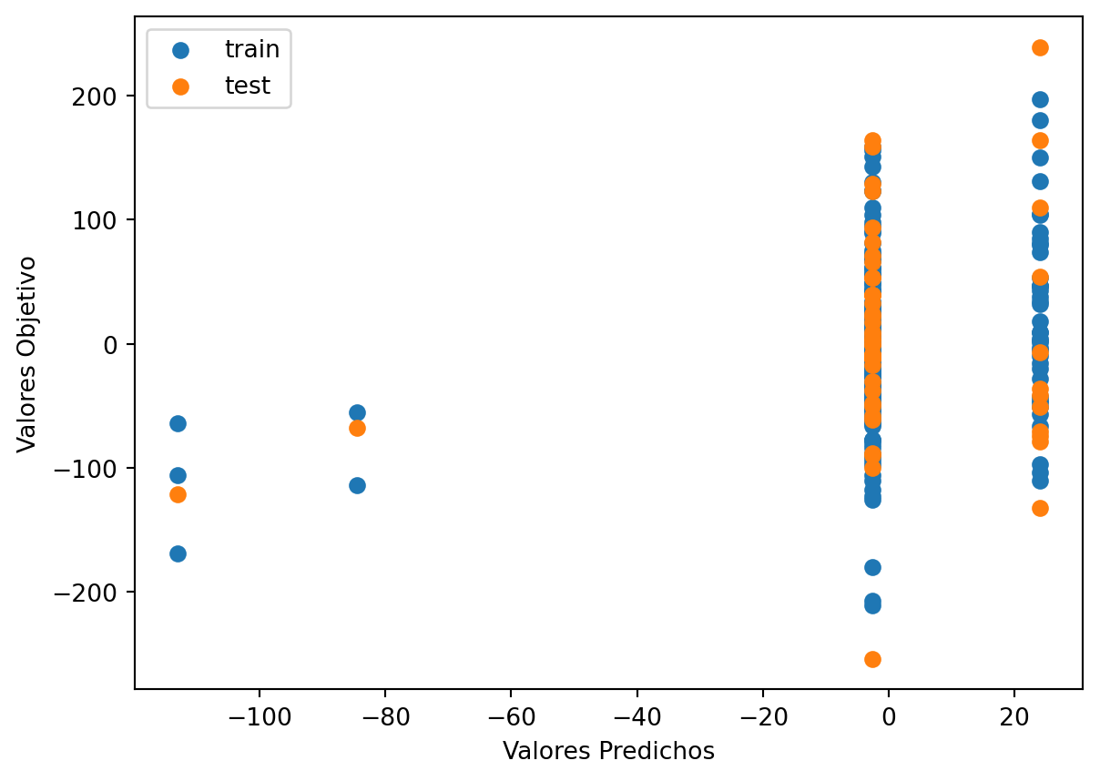

Raíz de la Pérdida cuadrática Entrenamiento: 63.56081240941628
Raíz de la Pérdida cuadrática Prueba: 82.96550957878867

Code

from sklearn import tree

listacaract=list(df1_Ori.columns.values)
respuesta=listacaract.pop()
text_representation = tree.export_text(decision_tree_Orig)
print(text_representation)

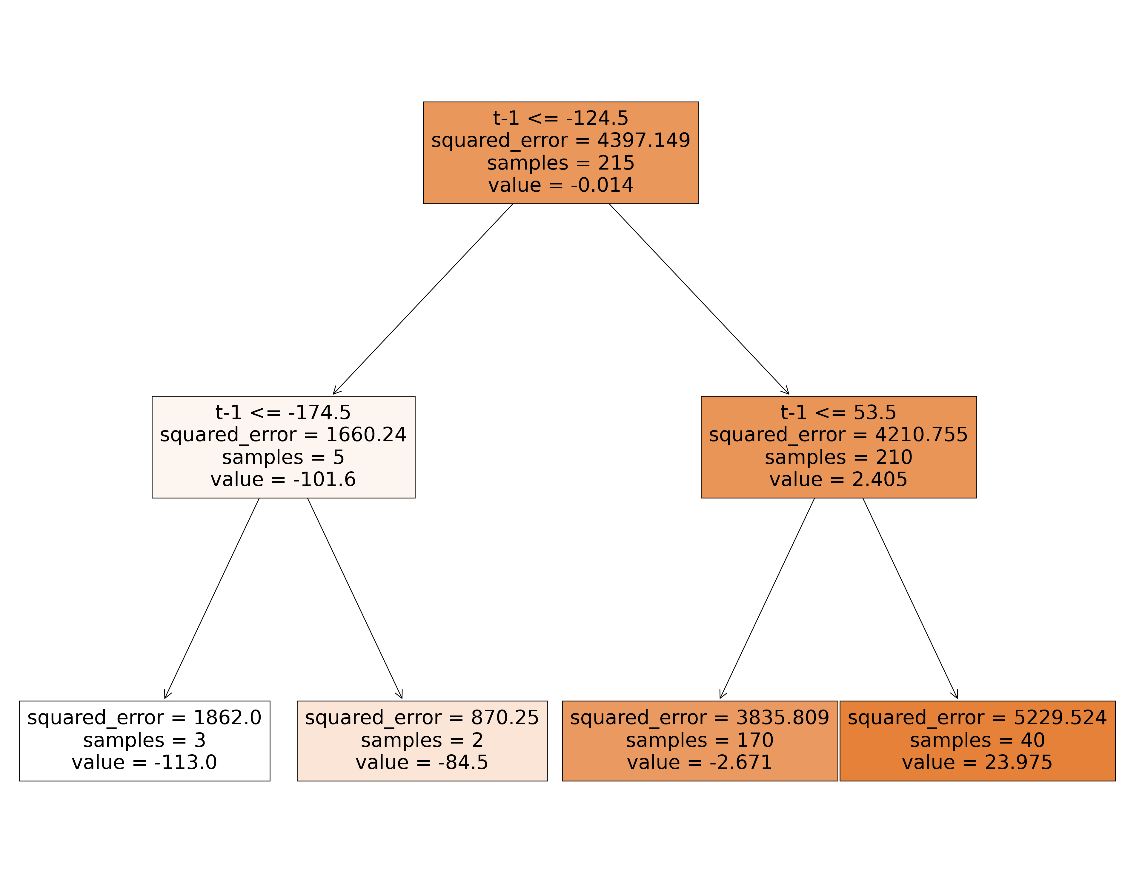
|--- feature_0 <= -124.50
|   |--- feature_0 <= -174.50
|   |   |--- value: [-113.00]
|   |--- feature_0 >  -174.50
|   |   |--- value: [-84.50]
|--- feature_0 >  -124.50
|   |--- feature_0 <= 53.50
|   |   |--- value: [-2.67]
|   |--- feature_0 >  53.50
|   |   |--- value: [23.98]

Code

fig = plt.figure(figsize=(25,20))
_ = tree.plot_tree(decision_tree_Orig, 
                   feature_names=listacaract,  
                   class_names=[respuesta],
                   filled=True)

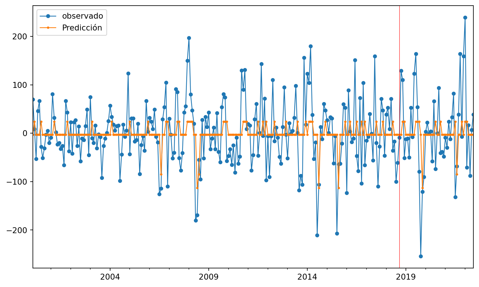
Ahora miraremos las predicciones comparadas con los valores verdaderos, para ver más claro lo anterior.

Code

print(train_val_prediction.size)
print(train_val_target.size)

print(test_prediction.size)
print(test_target.size)

Code

indicetrian_val_test=df1_Ori.index
print(indicetrian_val_test.size)  ###Tamaño del índice
indicetrain_val=indicetrian_val_test[0:215]
indicetest=indicetrian_val_test[215:269]

Code

print(indicetrain_val.size)
print(indicetest.size)

215
54

Code

targetjoint=np.concatenate((train_val_target,test_target))
predictionjoint=np.concatenate((train_val_prediction,test_prediction))
print(targetjoint.size)
print(predictionjoint.size)

269
269

Code

d = {'observado': targetjoint, 'Predicción': predictionjoint}
ObsvsPred1=pd.DataFrame(data=d,index=indicetrian_val_test)
ObsvsPred1.tail(54)

	observado	Predicción
2018-01-31	39.0	-2.670588
2018-02-28	53.0	-2.670588
2018-03-31	9.0	-2.670588
2018-04-30	71.0	-2.670588
2018-05-31	-36.0	23.975000
2018-06-30	-17.0	-2.670588
2018-07-31	-100.0	-2.670588
2018-08-31	-61.0	-2.670588
2018-09-30	-9.0	-2.670588
2018-10-31	129.0	-2.670588
2018-11-30	110.0	23.975000
2018-12-31	-51.0	23.975000
2019-01-31	-12.0	-2.670588
2019-02-28	-11.0	-2.670588
2019-03-31	-50.0	-2.670588
2019-04-30	53.0	-2.670588
2019-05-31	-8.0	-2.670588
2019-06-30	123.0	-2.670588
2019-07-31	164.0	23.975000
2019-08-31	54.0	23.975000
2019-09-30	-79.0	23.975000
2019-10-31	-254.0	-2.670588
2019-11-30	-121.0	-113.000000
2019-12-31	-90.0	-2.670588
2020-01-31	3.0	-2.670588
2020-02-29	22.0	-2.670588
2020-03-31	-1.0	-2.670588
2020-04-30	4.0	-2.670588
2020-05-31	-58.0	-2.670588
2020-06-30	66.0	-2.670588
2020-07-31	-74.0	23.975000
2020-08-31	0.0	-2.670588
2020-09-30	94.0	-2.670588
2020-10-31	-41.0	23.975000
2020-11-30	-38.0	-2.670588
2020-12-31	-48.0	-2.670588
2021-01-31	-9.0	-2.670588
2021-02-28	-30.0	-2.670588
2021-03-31	24.0	-2.670588
2021-04-30	-12.0	-2.670588
2021-05-31	33.0	-2.670588
2021-06-30	82.0	-2.670588
2021-07-31	-132.0	23.975000
2021-08-31	-68.0	-84.500000
2021-09-30	39.0	-2.670588
2021-10-31	164.0	-2.670588
2021-11-30	-7.0	23.975000
2021-12-31	159.0	-2.670588
2022-01-31	239.0	23.975000
2022-02-28	-71.0	23.975000
2022-03-31	17.0	-2.670588
2022-04-30	-88.0	-2.670588
2022-05-31	7.0	-2.670588
2022-06-30	39.0	-2.670588

Code

#gráfico
ax = ObsvsPred1['observado'].plot(marker="o", figsize=(10, 6), linewidth=1, markersize=4)  # Ajusta el grosor de las líneas y puntos
ObsvsPred1['Predicción'].plot(marker="o", linewidth=1, markersize=2, ax=ax)  # Ajusta el grosor de las líneas y puntos
# Agrega una línea vertical roja
ax.axvline(x=indicetrian_val_test[223].date(), color='red', linewidth=0.5)  # Ajusta el grosor de la línea vertical
# Muestra una leyenda
plt.legend()
plt.show()

Volver arriba